# Nelson-Siegel, Diebold-Li yield and Diebold-Rudebusch-Aruoba curve forecasting model
# By Cren
# -----------
## Loading required packages
library(YieldCurve, pos=4) ; library(quantmod, pos=4) ; library(ggplot2, pos=4) ; library(FitAR, pos=4) ; library(forecast, pos=4) ; library(vars, pos=4) ; library(timeSeries, pos=4)
# -----------
## Nelson-Siegel fitting
### Put R Var yield time series matrix as "X" (comprehensive of date rows and columns maturities); creating empty parameters' matrix
pnames <- c("beta_0", "beta_1", "beta_2", "lambda") ; param <- matrix(0, nrow = dim(X)[1], ncol = 4, dimnames = list(NULL, pnames)) ; param
### Fitting Nelson-Siegel model
for(i in 1:dim(X)[1]) {beta <- Nelson.Siegel(rate = X[i,], maturity = c(seq(from = 1, to = 10, by = 1), 15, 20, 30) * 12, MidTau = c(3, 5, 7) * 12) ; param[i,] <- t(beta)}
plot(as.timeSeries(param), main = "BTPs' Nelson-Siegel parameters", xlab = "Monthly observations from 28/2/2003 to 30/3/2012") ; grid(nx = 20, ny = 20)
# -----------
## Diebold-Li forecasting
### Augmented-Dickey-Fuller unit root test for each parameter
for(i in 1:4) {print(summary(ur.df(param[,i], type = "drift", lags = 1)))}
### Fitting AR(1) model (you can use "stats" or "FitAR" package according to your taste)
ar.beta <- matrix(0, nrow = 1, ncol = 4)
for(i in 1:4) {k <- FitARp(param[,i], 1, lag.max = 1, MLEQ = FALSE) ; ar.beta[,i] <- predict(k, n.ahead = 1)$Forecasts[1]}
for(i in 1:4) {k <- ar(x = param[,i], aic = FALSE, order.max = 1, demean = TRUE) ; ar.beta[,i] <- predict(k, n.ahead = 1)$pred[1]}
### Yield curve forecasting via AR(1) model
y_1 <- NSrates(betaCoeff = param[dim(X)[1],1:3], lambdat = param[dim(X)[1],4], maturity = c(seq(from = 1, to = 10, by = 1), 15, 20, 30) * 12) ; y_1 ; y <- NSrates(betaCoeff = ar.beta[,1:3], lambdat = ar.beta[4], maturity = c(seq(from = 1, to = 10, by = 1), 15, 20, 30) * 12) ; y ; Maturity <- c(seq(from = 1, to = 10, by = 1), 15, 20, 30) * 1 ; Maturity
plot(lwd = 2, X[dim(X)[1],] ~ Maturity, main = "Diebold-Li BTPs' yield curve prediction", ylab = "Yield [%]", xlab = "Maturity [years]", type = "b") ; lines(lwd = 2, Maturity, y, col = 2) ; lines(lwd = 2, Maturity, y_1, col = 3) ; grid(nx = 20, ny = 20) ; legend(lwd = c(2, 2, 2), col = c(1, 2, 3), bty = "n", x = "bottomright", legend = c("Actual yield curve", "1 month forecasted yield curve", "Actual Nelson-Siegel fitting"))
# -----------
## Diebold-Rudebusch-Aruoba forecasting
### ECST IT Bloomberg's function for Italy Economic Statistics: ITPRNIY Index | EURR003M Index | CPTFEMU Index
### Coercing lambda to...
param[,4] <- max(param[,4])
param[,4] <- 0.069 # Diebold-Li's choice
### Put R Var economic variables as "Y". Creating VAR data matrix and estimating VAR model (neither constant nor trend); 1-step forecast
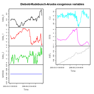
L <- cbind(param[,1:3], Y) ; plot(as.timeSeries(L), plot.type = "m", col = c(1,2,3,4,5,6), main = "Diebold-Rudebusch-Aruoba exogenous variables")
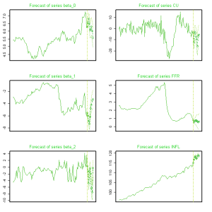
var.2c <- VAR(L, p = 48, type = "none", season = NULL, exogen = NULL, lag.max = 48, ic = "AIC") ; var.2d <- restrict(var.2c, method = "ser", thresh = 2.0) ; var.2c.prd <- predict(var.2d, n.ahead = 1, ci = 0.9) ; var.2c.prd ; par(mai = c(0.5,0.5,0.5,0.5))
plot(var.2c.prd, ylab = "", col = terrain.colors(12), lwd = 1, type = "o", pch = 23, col.main = "green3", xaxt = "n", font.main = "1")
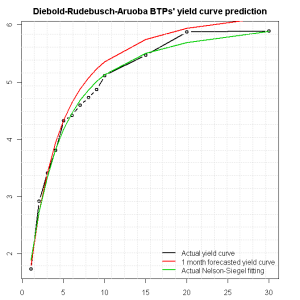
### Yield curve forecasting
DRApar <- matrix(0, nrow = 1, ncol = 3) ; DRApar[1] <- var.2c.prd$fcst$beta_0[1] ; DRApar[2] <- var.2c.prd$fcst$beta_1[1] ; DRApar[3] <- var.2c.prd$fcst$beta_2[1] ; DRApar
y_DRA <- NSrates(betaCoeff = DRApar, lambdat = param[1,4], maturity = c(seq(from = 1, to = 10, by = 1), 15, 20, 30) * 12)
plot(lwd = 2, X[dim(X)[1],] ~ Maturity, main = "Diebold-Rudebusch-Aruoba BTPs' yield curve prediction", ylab = "Yield [%]", xlab = "Maturity [years]", type = "b") ; lines(lwd = 2, Maturity, y_DRA, col = 2) ; lines(lwd = 2, Maturity, y_1, col = 3) ; grid(nx = 20, ny = 20) ; legend(lwd = c(2, 2, 2), col = c(1, 2, 3), bty = "n", x = "bottomright", l
")